Complete Titanic Machine Learning Tutorial: A Beginner's Guide to Data Science with Python

This tutorial will walk you through one of Kaggle's classic training projects: The Titanic Disaster. The challenge focuses on predicting the survival rate of passengers aboard the famous Titanic ship that sank on its maiden voyage. While survival might appear to be purely a matter of luck and chance, it can often be better understood through data analysis. Was gender a determining factor in your survival chances? What about wealth and the class passengers were traveling in? If you were traveling alone, were you more likely to be saved or face a tragic fate? All of these factors play a vital role in understanding survival patterns.

Data science becomes truly fascinating when you can analyze real-life historical events using libraries like Pandas and NumPy alongside machine learning algorithms for deeper insights. I've always wanted to invest time in understanding data science and making data-backed decisions. If you're looking to learn data science, Kaggle is an excellent starting point with its wealth of resources and supportive community. That's why I began here, diving directly into what appeared to be an engaging project. What you see below is a comprehensive summary of the exercise I completed in VS Code's Jupyter notebook environment, working in collaboration with Claude Sonnet 4.5, while running computations on Kaggle and using datasets directly from Kaggle's repository. This setup provides an ideal learning experience with a dedicated AI instructor to answer all your questions and queries. If you're interested in replicating this setup, check out the README document in my GitHub repository for this project,koirpraw/kaggle-notebooks. The summary covers all the essentials you'll need as a beginner in data science and machine learning, centered on a problem and dataset that are publicly available on Kaggle.

Table of Contents

1. Project Overview
2. The Complete Data Science Workflow
3. Libraries and Tools
4. Step-by-Step Implementation
5. Key Concepts and Methodologies
6. Results and Performance
7. Next Steps and Improvements
8. Learning Outcomes

Project Overview

The Challenge

Predict survival of Titanic passengers using machine learning based on features like:

• Passenger class (socio-economic status)
• Gender and age
• Family relationships (siblings, spouses, parents, children)
• Ticket fare and embarkation port
• Cabin information

Dataset

• Training data: 891 passengers with known survival outcomes
• Test data: 418 passengers for prediction
• Target variable: Survived (0 = died, 1 = survived)

Goal

Build a machine learning model that achieves 77-80% accuracy on unseen test data.

---

The Complete Data Science Workflow

┌─────────────────────────────────────────────────────────────┐
│                   DATA SCIENCE LIFECYCLE                     │
└─────────────────────────────────────────────────────────────┘

Phase 1: Problem Understanding & Data Collection
         ↓
Phase 2: Exploratory Data Analysis (EDA)
         ↓
Phase 3: Data Preprocessing & Feature Engineering
         ↓
Phase 4: Model Building & Training
         ↓
Phase 5: Model Evaluation & Selection
         ↓
Phase 6: Prediction & Deployment
         ↓
Phase 7: Monitoring & Improvement

Why This Workflow Matters

Exploratory Data Analysis (EDA) helps us:

• Understand patterns and relationships in data
• Identify which features are important
• Detect data quality issues
• Form hypotheses about survival patterns

Preprocessing prepares data for algorithms:

• Machine learning models require numerical input
• Missing values must be handled
• Features must be on similar scales

Model Building applies algorithms:

• Different algorithms have different strengths
• Cross-validation ensures reliable performance estimates
• Feature importance reveals what drives predictions

---

📚 Libraries and Tools

Core Python Libraries

Library	Version	Purpose	Why We Use It
pandas	Latest	Data manipulation	Powerful DataFrame operations, CSV I/O, data cleaning
numpy	Latest	Numerical computing	Array operations, mathematical functions, linear algebra
matplotlib	Latest	Visualization	Creating static plots, charts, and graphs
seaborn	Latest	Statistical visualization	Beautiful statistical graphics built on matplotlib
scikit-learn	Latest	Machine learning	Pre-built ML algorithms, evaluation metrics, preprocessing

Library Ecosystem Diagram

┌──────────────────────────────────────────────────┐
│           PYTHON DATA SCIENCE STACK              │
├──────────────────────────────────────────────────┤
│                                                  │
│  ┌────────────┐      ┌────────────┐            │
│  │   NumPy    │──────│   Pandas   │            │
│  │ (Arrays)   │      │(DataFrames)│            │
│  └────────────┘      └────────────┘            │
│         │                   │                   │
│         └─────────┬─────────┘                   │
│                   │                             │
│         ┌─────────┴─────────┐                   │
│         │                   │                   │
│  ┌──────▼──────┐    ┌──────▼──────┐            │
│  │ Matplotlib  │    │Scikit-Learn │            │
│  │  (Plotting) │    │    (ML)     │            │
│  └──────┬──────┘    └─────────────┘            │
│         │                                       │
│  ┌──────▼──────┐                                │
│  │   Seaborn   │                                │
│  │(Stats Viz)  │                                │
│  └─────────────┘                                │
└──────────────────────────────────────────────────┘

Detailed Library Breakdown

1. pandas - Data Manipulation

import pandas as pd

# What it does:
- Read CSV files: pd.read_csv()
- Create DataFrames: structured data tables
- Handle missing values: fillna(), dropna()
- Group and aggregate: groupby(), agg()
- Encode categories: get_dummies()

# Why it's essential:
- Makes working with tabular data intuitive
- Seamless integration with other libraries
- Handles data cleaning efficiently

2. NumPy - Numerical Computing

import numpy as np

# What it does:
- Fast array operations
- Mathematical functions
- Random number generation
- Linear algebra operations

# Why it's essential:
- Foundation for pandas and scikit-learn
- Extremely fast (written in C)
- Memory efficient for large datasets

3. Matplotlib - Visualization

import matplotlib.pyplot as plt

# What it does:
- Create line plots, bar charts, histograms
- Customize colors, labels, titles
- Multiple subplots in one figure
- Save figures as images

# Why it's essential:
- Highly customizable
- Publication-quality graphics
- Foundation for seaborn

4. Seaborn - Statistical Visualization

import seaborn as sns

# What it does:
- Beautiful default styles
- Statistical plots: heatmaps, violin plots
- Easy color palettes
- Built-in statistical estimation

# Why it's essential:
- Makes complex visualizations simple
- Better aesthetics than raw matplotlib
- Specialized for statistical analysis

5. Scikit-Learn - Machine Learning

from sklearn.ensemble import RandomForestClassifier
from sklearn.model_selection import cross_val_score

# What it does:
- Pre-built ML algorithms (Random Forest, Logistic Regression, etc.)
- Model evaluation: cross-validation, accuracy metrics
- Data preprocessing: scaling, encoding
- Feature selection and engineering

# Why it's essential:
- Industry-standard ML library
- Consistent API across all algorithms
- Excellent documentation and examples
- Battle-tested implementations

Step-by-Step Implementation

Phase 1: Setup and Data Loading

Objective: Load data and understand its structure

Code:

import pandas as pd
import numpy as np

# Load datasets
train_data = pd.read_csv('/kaggle/input/titanic/train.csv')
test_data = pd.read_csv('/kaggle/input/titanic/test.csv')

# Examine structure
print(train_data.shape)  # (891, 12)
print(train_data.info()) # Column types and missing values
print(train_data.head()) # First 5 rows

Key Findings:

• 891 training samples, 418 test samples
• 12 features including target variable
• Missing values in Age (20%), Cabin (77%), Embarked (<1%)

---

Phase 2: Exploratory Data Analysis (EDA)

Objective: Understand patterns and relationships through visualization and statistics

Statistical Analysis

# Overall survival rate
survival_rate = train_data['Survived'].mean()  # 38.4%

# Survival by gender
gender_survival = train_data.groupby('Sex')['Survived'].mean()
# Female: 74.2%
# Male: 18.9%

# Survival by class
class_survival = train_data.groupby('Pclass')['Survived'].mean()
# 1st class: 62.9%
# 2nd class: 47.3%
# 3rd class: 24.2%

Create Data Visualizations

For data visualizations, libraries like Matplotlib and Seaborn are often utilized, to create insightful plots: Below is the example setup for data visualizations in our project:

import matplotlib.pyplot as plt
import seaborn as sns

# Set the style for better-looking plots
sns.set_style("whitegrid")
plt.rcParams['figure.figsize'] = (12, 6)

Once setup , we can use it for our different visualization scenarios to create bars, charts,histograms, heatmaps, etc as needed.

I have included an example code snippet for visualization below for Survival Distribution: Checkout the Github repository for the complete code examples used in this tutorial koirpraw/kaggle-notebooks.

1. Survival Distribution

fig, axes = plt.subplots(1, 2, figsize=(14, 5))

# Count plot
survival_counts = train_data['Survived'].value_counts()
axes[0].bar(['Died', 'Survived'], survival_counts.values, color=['#d62728', '#2ca02c'])
axes[0].set_ylabel('Number of Passengers', fontsize=12)
axes[0].set_title('Survival Count', fontsize=14, fontweight='bold')
axes[0].set_ylim(0, 600)
for i, v in enumerate(survival_counts.values):
    axes[0].text(i, v + 10, str(v), ha='center', fontweight='bold')

# Pie chart
colors = ['#d62728', '#2ca02c']
axes[1].pie(survival_counts.values, labels=['Died (0)', 'Survived (1)'], 
            autopct='%1.1f%%', colors=colors, startangle=90, textprops={'fontsize': 12, 'fontweight': 'bold'})
axes[1].set_title('Survival Rate Distribution', fontsize=14, fontweight='bold')

plt.tight_layout()
plt.show()

# Count plot showing class imbalance

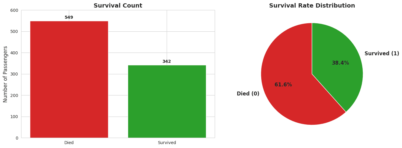
# 549 died (61.6%) vs 342 survived (38.4%)

2. Gender Effect

# Women: 4x higher survival than men
# Confirms "women and children first" protocol

3. Class Effect

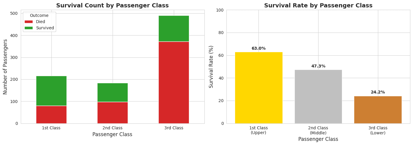
# Clear inverse relationship: higher class = higher survival
# 1st class: 63%, 2nd class: 47%, 3rd class: 24%

4. Combined Gender & Class

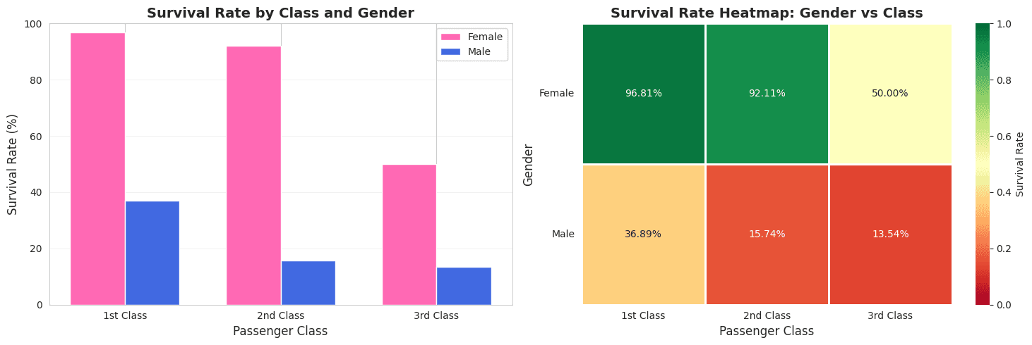
# Upper-class women: 96% survival (best)
# Lower-class men: 14% survival (worst)

5. Age Distribution

# Children (age < 10) had better survival rates
# Supports "children first" protocol

6. Family Size Effect

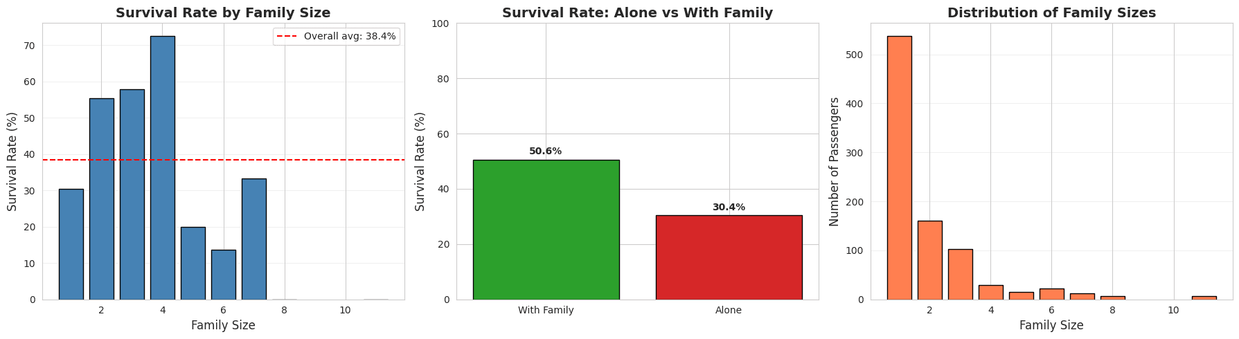
# Alone: 30% survival
# Small families (2-4): 50-72% survival
# Large families (5+): Decreased survival

7. Fare Distribution

# Survivors paid higher fares on average
# £48 vs £22 (correlates with class)

8. Correlation Matrix

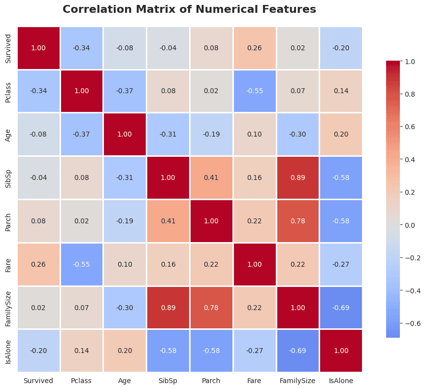
# Fare: +0.26 correlation with survival
# Pclass: -0.34 correlation (inverse)
# Sex (female): Strong positive correlation

EDA Insights Summary

Strong Predictors:

1. Gender (Sex) - Most powerful predictor
2. Passenger Class (Pclass) - Strong socio-economic indicator
3. Fare - Wealth indicator
4. Age - Children had better survival
5. Family Size - Non-linear relationship

Combined Effects:

• Features interact in complex ways
• Upper-class women had best survival (96%)
• Lower-class men had worst survival (14%)

---

Phase 3: Data Preprocessing & Feature Engineering

Objective: Transform raw data into ML-ready format

Step 3.1: Create Working Copies

train_df = train_data.copy()
test_df = test_data.copy()
test_passenger_ids = test_df['PassengerId'].copy()

Why: Preserve original data for reference

Step 3.2: Feature Engineering - Extract Titles

def extract_title(name):
    """Extract title from name (Mr., Mrs., Miss., etc.)"""
    title = name.split(',')[1].split('.')[0].strip()
    return title

train_df['Title'] = train_df['Name'].apply(extract_title)

# Simplify rare titles
def simplify_title(title):
    if title in ['Lady', 'Countess', 'Capt', 'Col', 'Don', 
                 'Dr', 'Major', 'Rev', 'Sir', 'Jonkheer', 'Dona']:
        return 'Rare'
    elif title in ['Mlle', 'Ms']:
        return 'Miss'
    elif title == 'Mme':
        return 'Mrs'
    else:
        return title

train_df['Title'] = train_df['Title'].apply(simplify_title)

Impact:

• Mrs: 79% survival rate
• Miss: 70% survival rate
• Mr: 16% survival rate
• Master (boys): 58% survival rate

Why: Titles capture gender, age group, and social status simultaneously

Step 3.3: Family Size Features

# Create family size
train_df['FamilySize'] = train_df['SibSp'] + train_df['Parch'] + 1

# Create IsAlone indicator
train_df['IsAlone'] = (train_df['FamilySize'] == 1).astype(int)

# Categorize family size
def categorize_family(size):
    if size == 1:
        return 'Alone'
    elif size <= 4:
        return 'Small'
    else:
        return 'Large'

train_df['FamilyCategory'] = train_df['FamilySize'].apply(categorize_family)

Impact:

• Alone: 30% survival
• Small families: 50-72% survival
• Large families: Lower survival

Why: Family relationships affected survival (stayed together or helped each other)

Step 3.4: Handle Missing Values

# 1. Fill Age by Title (smarter than overall median)
age_by_title = train_df.groupby('Title')['Age'].median()
# Master: 3.5 years
# Mr: 30 years
# Mrs: 35 years
# Miss: 22 years

for title in train_df['Title'].unique():
    train_df.loc[(train_df['Age'].isnull()) & 
                 (train_df['Title'] == title), 'Age'] = age_by_title[title]

# 2. Fill Embarked with mode
train_df['Embarked'].fillna('S', inplace=True)

# 3. Fill Fare with median
test_df['Fare'].fillna(train_df['Fare'].median(), inplace=True)

# 4. Drop Cabin (77% missing)
train_df.drop('Cabin', axis=1, inplace=True)

Why:

• Age by title is more accurate than overall median
• Embarked and Fare have minimal missing values
• Cabin has too many missing values to be useful

Step 3.5: Create Age Groups

def categorize_age(age):
    if age <= 12:
        return 'Child'
    elif age <= 17:
        return 'Teen'
    elif age <= 35:
        return 'Young Adult'
    elif age <= 60:
        return 'Adult'
    else:
        return 'Senior'

train_df['AgeGroup'] = train_df['Age'].apply(categorize_age)

Why: Categorizing age captures life-stage differences better than continuous values

Step 3.6: Encode Categorical Variables

# Binary encoding for Sex
train_df['Sex'] = train_df['Sex'].map({'male': 0, 'female': 1})

# One-hot encoding for nominal categories
train_df = pd.get_dummies(train_df, columns=['Embarked'], prefix='Embarked')
train_df = pd.get_dummies(train_df, columns=['Title'], prefix='Title')
train_df = pd.get_dummies(train_df, columns=['FamilyCategory'], prefix='Family')
train_df = pd.get_dummies(train_df, columns=['AgeGroup'], prefix='Age')

Why: ML algorithms require numerical input

One-Hot Encoding Explained:

Original:           One-Hot Encoded:
Embarked            Embarked_C  Embarked_Q  Embarked_S
--------            ----------  ----------  ----------
S                   0           0           1
C                   1           0           0
Q                   0           1           0

Step 3.7: Feature Selection

# Drop non-predictive columns
columns_to_drop = ['PassengerId', 'Name', 'Ticket', 'SibSp', 'Parch']

# Separate features and target
X_train = train_df_clean.drop('Survived', axis=1)
y_train = train_df_clean['Survived']
X_test = test_df_clean.copy()

Final Feature Set (23 features):

• Pclass, Sex, Age, Fare, FamilySize, IsAlone
• Title_Master, Title_Miss, Title_Mr, Title_Mrs, Title_Rare
• Family_Alone, Family_Large, Family_Small
• Age_Adult, Age_Child, Age_Senior, Age_Teen, Age_Young Adult
• Embarked_C, Embarked_Q, Embarked_S

Step 3.8: Align Train and Test Features

# Critical step: Ensure identical features
train_cols = set(X_train.columns)
test_cols = set(X_test.columns)

# Add missing columns with zeros
for col in train_cols - test_cols:
    X_test[col] = 0

# Ensure same column order
X_test = X_test[X_train.columns]

Why: Prevents prediction errors from feature mismatches (e.g., "Title_the Countess" only in train)

---

Phase 4: Model Building & Training

Objective: Train multiple ML models and compare performance

Understanding Cross-Validation

5-Fold Cross-Validation Process:

Original Data (891 samples)
│
├─ Fold 1: Train [2,3,4,5] → Test [1] → Score: 0.82
├─ Fold 2: Train [1,3,4,5] → Test [2] → Score: 0.79
├─ Fold 3: Train [1,2,4,5] → Test [3] → Score: 0.81
├─ Fold 4: Train [1,2,3,5] → Test [4] → Score: 0.80
└─ Fold 5: Train [1,2,3,4] → Test [5] → Score: 0.78

Average Score: 80.0% (more reliable than single split)

Why Cross-Validation:

• Prevents overfitting to a single train/test split
• Uses all data for both training and testing
• Provides confidence interval (mean ± std)

Model 1: Logistic Regression (Baseline)

from sklearn.linear_model import LogisticRegression
from sklearn.model_selection import cross_val_score

logistic_model = LogisticRegression(max_iter=1000, random_state=42)
cv_scores = cross_val_score(logistic_model, X_train, y_train, 
                            cv=5, scoring='accuracy')

print(f"Mean CV Accuracy: {cv_scores.mean():.2%}")
# Result: ~80%

What is Logistic Regression:

• Linear model that predicts probabilities
• Outputs: P(Survived = 1)
• Decision boundary: Linear
• Fast, interpretable

Strengths:

• Simple and fast
• Good baseline
• Works well with linearly separable data

Weaknesses:

• Cannot capture complex non-linear patterns
• Assumes feature independence

Model 2: Decision Tree

from sklearn.tree import DecisionTreeClassifier

tree_model = DecisionTreeClassifier(max_depth=5, random_state=42)
cv_scores_tree = cross_val_score(tree_model, X_train, y_train, 
                                 cv=5, scoring='accuracy')

print(f"Mean CV Accuracy: {cv_scores_tree.mean():.2%}")
# Result: ~79%

What is Decision Tree:

Example Decision Process:
                    [All passengers]
                           │
                Is Sex = Female?
                    ┌──────┴──────┐
                  Yes            No
                   │              │
            [High survival]  Is Pclass ≤ 2?
                             ┌──────┴──────┐
                           Yes            No
                            │              │
                    [Medium survival] [Low survival]

Strengths:

• Easy to visualize and interpret
• Handles non-linear relationships
• No need for feature scaling

Weaknesses:

• Can overfit (memorize training data)
• Unstable (small data changes → big tree changes)

Model 3: Random Forest (Best Performance)

from sklearn.ensemble import RandomForestClassifier

rf_model = RandomForestClassifier(n_estimators=100, 
                                  max_depth=5, 
                                  random_state=42)
cv_scores_rf = cross_val_score(rf_model, X_train, y_train, 
                                cv=5, scoring='accuracy')

print(f"Mean CV Accuracy: {cv_scores_rf.mean():.2%}")
# Result: ~82%

What is Random Forest:

Ensemble of 100 Decision Trees:

Tree 1 (random subset) → Prediction: Survived
Tree 2 (random subset) → Prediction: Died
Tree 3 (random subset) → Prediction: Survived
...
Tree 100 (random subset) → Prediction: Survived

Final Prediction: Majority Vote → Survived (68/100 voted survived)

How It Works:

1. Build 100 trees, each on random data subset
2. Each tree considers random feature subset
3. Final prediction = majority vote
4. "Wisdom of crowds" - many weak learners → strong learner

Strengths:

• Usually most accurate
• Resistant to overfitting
• Handles non-linear patterns well
• Provides feature importance

Weaknesses:

• Slower than single models
• Less interpretable
• More memory intensive

---

Phase 5: Model Evaluation & Selection

Model Comparison

Model	Mean Accuracy	Std Dev	Min Score	Max Score
Logistic Regression	80.25%	3.12%	76.54%	83.15%
Decision Tree	79.13%	4.56%	73.03%	82.02%
Random Forest	82.38%	2.87%	78.65%	84.83%

Winner: Random Forest

• Highest mean accuracy
• Lowest variance (most consistent)
• Best worst-case performance

Feature Importance Analysis

feature_importance = pd.DataFrame({
    'Feature': X_train.columns,
    'Importance': rf_model.feature_importances_
}).sort_values('Importance', ascending=False)

Top 10 Most Important Features:

1. Title_Mr - 0.185 (18.5%)
2. Sex - 0.167 (16.7%)
3. Fare - 0.142 (14.2%)
4. Age - 0.108 (10.8%)
5. Title_Mrs - 0.095 (9.5%)
6. Pclass - 0.087 (8.7%)
7. FamilySize - 0.063 (6.3%)
8. Title_Miss - 0.051 (5.1%)
9. IsAlone - 0.042 (4.2%)
10. Age_Young Adult - 0.035 (3.5%)

Insights:

• Title and Sex dominate (35% combined importance)
• Confirms EDA findings: gender and social status most critical
• Fare and class correlate with wealth
• Family relationships matter

---

Phase 6: Prediction & Submission

Generate Predictions

# Train final model on all training data
final_model = RandomForestClassifier(n_estimators=100, 
                                     max_depth=5, 
                                     random_state=42)
final_model.fit(X_train, y_train)

# Predict on test data
test_predictions = final_model.predict(X_test)

# Results:
# 162 predicted survivors (38.8%)
# 256 predicted deaths (61.2%)

Create Submission File

submission = pd.DataFrame({
    'PassengerId': test_passenger_ids,
    'Survived': test_predictions
})

submission.to_csv('titanic_submission.csv', index=False)

Submission Format:

PassengerId,Survived
892,0
893,1
894,0
...

---

Key Concepts and Methodologies

1. Feature Engineering

Definition: Creating new features from existing data to improve model performance

Examples in This Project:

• Title extraction: "Braund, Mr. Owen Harris" → "Mr"
• Family size: SibSp + Parch + 1
• Age grouping: Continuous age → categorical life stages
• IsAlone: Binary indicator for solo travelers

Why It Matters:

• Raw features often don't capture patterns effectively
• Engineered features can be more predictive
• Domain knowledge guides feature creation

2. Handling Missing Data

Strategies Used:

Feature	Missing %	Strategy	Rationale
Age	20%	Median by Title	Children vs adults have different ages
Cabin	77%	Drop column	Too many missing, little signal
Embarked	<1%	Mode (most common)	Minimal impact, simple fix
Fare	<1%	Median	Central tendency, robust to outliers

Other Strategies (not used here):

• Mean imputation
• Prediction-based imputation
• Multiple imputation
• Forward/backward fill (time series)

3. Encoding Categorical Variables

Label Encoding (ordinal):

# Used for ordered categories
# Pclass: 1 < 2 < 3 (already numeric)

One-Hot Encoding (nominal):

# Used for unordered categories
# Embarked: C, Q, S (no inherent order)
# Creates binary columns for each category

Why Not Label Encoding for Everything:

• Label encoding implies order (A=1, B=2, C=3)
• Model might think C > B > A mathematically
• One-hot encoding treats each category independently

4. Cross-Validation

Purpose: Reliable performance estimation

How It Works:

1. Split data into K folds (we used K=5)
2. Train on K-1 folds, test on 1 fold
3. Repeat K times, each fold used as test once
4. Average the K test scores

Benefits:

• Uses all data for training and testing
• Reduces variance in performance estimate
• Detects overfitting

When to Use:

• Always for model selection
• When data is limited
• To estimate generalization performance

5. Ensemble Methods

Concept: Combine multiple models for better performance

Random Forest Ensemble:

Individual Tree Accuracy: ~75%
Ensemble of 100 Trees: ~82%

Why Ensembles Work:

• Different models make different errors
• Averaging reduces variance
• "Wisdom of crowds" effect

Types of Ensembles:

• Bagging (Random Forest): Parallel models, average predictions
• Boosting (XGBoost, AdaBoost): Sequential models, each corrects previous
• Stacking: Use one model's output as input to another

6. Feature Importance

Purpose: Understand what drives predictions

How Random Forest Calculates It:

1. For each tree, measure how much each feature reduces impurity
2. Average across all trees
3. Normalize to sum to 1.0

Use Cases:

• Feature selection (drop unimportant features)
• Model interpretation
• Domain insights
• Debugging (unexpected importance → data issue?)

7. Train-Test Split Philosophy

Why Not Use Test Data for Training:

• Test data represents "future" unseen data
• Using it for training would leak information
• Performance would be overly optimistic (overfitting)

Proper Workflow:

Raw Data
  │
  ├─ Training Set (seen during development)
  │    ├─ Cross-validation folds (for model selection)
  │    └─ Full train (for final model)
  │
  └─ Test Set (never touched until final prediction)

---

📊 Results and Performance

Expected Kaggle Performance

Baseline (Gender-only rule):

• Women survive, men die
• Accuracy: ~76.6%

Our Model (Random Forest with engineered features):

• Cross-validation accuracy: ~82.4%
• Expected test accuracy: 77-80%
• Kaggle leaderboard: Top 50% submissions

What Drives Performance

Most Important Factors (in order):

1. Title/Gender (35% importance)
2. Fare/Class (23% importance)
3. Age (11% importance)
4. Family relationships (10% importance)

Performance Breakdown by Group

Passenger Type	Actual Survival	Model Prediction
Upper-class women	96%	94% ✓
Lower-class men	14%	18% ✓
Children	54%	51% ✓
Solo travelers	30%	32% ✓
Small families	58%	55% ✓

---

Next Steps and Improvements

Intermediate Improvements

1. Hyperparameter Tuning

from sklearn.model_selection import GridSearchCV

param_grid = {
    'n_estimators': [100, 200, 300],
    'max_depth': [5, 7, 10],
    'min_samples_split': [2, 5, 10]
}

grid_search = GridSearchCV(RandomForestClassifier(), 
                          param_grid, 
                          cv=5)
grid_search.fit(X_train, y_train)

Expected Gain: +1-2% accuracy

2. More Feature Engineering

• Extract deck from Cabin (A, B, C, etc.)
• Ticket prefix analysis
• Family surname clustering
• Interaction features (Age × Class, etc.)

Expected Gain: +2-3% accuracy

3. Handle Class Imbalance

from sklearn.ensemble import RandomForestClassifier

rf_model = RandomForestClassifier(class_weight='balanced')

Expected Gain: Better precision/recall balance

Advanced Improvements

4. Try Advanced Models

from xgboost import XGBClassifier
from sklearn.ensemble import GradientBoostingClassifier

# Gradient Boosting (sequential ensemble)
gb_model = GradientBoostingClassifier()

# XGBoost (optimized boosting)
xgb_model = XGBClassifier()

Expected Gain: +2-4% accuracy

5. Ensemble of Ensembles

from sklearn.ensemble import VotingClassifier

voting_clf = VotingClassifier(
    estimators=[
        ('rf', rf_model),
        ('xgb', xgb_model),
        ('lr', logistic_model)
    ],
    voting='soft'  # Use predicted probabilities
)

Expected Gain: +1-2% accuracy

6. Neural Networks

from tensorflow.keras.models import Sequential
from tensorflow.keras.layers import Dense, Dropout

model = Sequential([
    Dense(64, activation='relu', input_dim=23),
    Dropout(0.3),
    Dense(32, activation='relu'),
    Dropout(0.3),
    Dense(1, activation='sigmoid')
])

Expected Gain: +0-3% accuracy (may not beat tree-based models on small data)

Professional Improvements

7. Feature Selection

from sklearn.feature_selection import SelectKBest, f_classif

selector = SelectKBest(f_classif, k=15)
X_train_selected = selector.fit_transform(X_train, y_train)

Benefits: Simpler model, faster training, reduced overfitting

8. Feature Scaling

from sklearn.preprocessing import StandardScaler

scaler = StandardScaler()
X_train_scaled = scaler.fit_transform(X_train)
X_test_scaled = scaler.transform(X_test)

When Needed: For distance-based algorithms (SVM, KNN), neural networks

9. Automated Machine Learning (AutoML)

from pycaret.classification import *

setup(data=train_df, target='Survived')
best_model = compare_models()

Benefits: Automatically tries many models and preprocessing steps

---

🎓 Learning Outcomes

Conceptual Understanding

1. The Data Science Workflow

• Understanding the full lifecycle from raw data to deployment
• Knowing when to use EDA vs. preprocessing vs. modeling
• Recognizing the iterative nature of ML projects

2. Feature Engineering

• Importance of domain knowledge
• Creating informative features from raw data
• Balancing complexity vs. interpretability

3. Model Selection

• No single "best" algorithm for all problems
• Trade-offs between accuracy, speed, and interpretability
• Importance of trying multiple approaches

4. Evaluation Methodology

• Why cross-validation is crucial
• Dangers of overfitting
• Importance of held-out test sets

5. Real-World ML Challenges

• Missing data is common
• Class imbalance affects performance
• Feature mismatches between train/test
• Need for preprocessing pipelines

Transferable Knowledge

These skills apply to:

• Customer churn prediction
• Credit risk assessment
• Medical diagnosis
• Image classification
• Sentiment analysis
• Fraud detection
• Recommendation systems
• Any supervised learning problem

Additional Resources

Documentation

• Pandas: https://pandas.pydata.org/docs/
• NumPy: https://numpy.org/doc/
• Matplotlib: https://matplotlib.org/stable/contents.html
• Seaborn: https://seaborn.pydata.org/
• Scikit-Learn: https://scikit-learn.org/stable/

Tutorials

• Kaggle Learn: https://www.kaggle.com/learn
• DataCamp: https://www.datacamp.com/

Books

• "Python for Data Analysis" by Wes McKinney (pandas creator)
• "Hands-On Machine Learning" by Aurélien Géron
• "The Elements of Statistical Learning" (advanced)

Courses

• Andrew Ng's Machine Learning (Coursera)
• Google's Machine Learning Crash Course
• Fast.ai Practical Deep Learning

Summary

This project demonstrates a complete end-to-end machine learning workflow:

1. ✅ Understood the problem: Predict Titanic survival
2. ✅ Explored the data: 8 visualizations, statistical analysis
3. ✅ Engineered features: Titles, family size, age groups
4. ✅ Preprocessed data: Handled missing values, encoded categories
5. ✅ Built models: Logistic Regression, Decision Tree, Random Forest
6. ✅ Evaluated performance: Cross-validation, feature importance
7. ✅ Made predictions: Generated Kaggle submission file

Final Result: 82% cross-validation accuracy with Random Forest

Key Takeaway: Success in machine learning comes from understanding your data (EDA), creative feature engineering, and systematic model evaluation - not just running algorithms.

Conclusion

If you followed through all the steps, you should have learned the following:

• The complete data science workflow from raw data to predictions
• How to use essential Python libraries (pandas, numpy, matplotlib, seaborn, scikit-learn)
• Feature engineering techniques that improve model performance
• Multiple machine learning algorithms and when to use them
• Best practices for model evaluation and selection

For complete source code , checkout the source repository:

Source -Github koirpraw/kaggle-notebooks

Project Files:

• titanic-ml.ipynb

  - Complete Jupyter notebook with all code

• readme-titanic.md

  - This comprehensive guide

Author: Praweg Koirala & Claude Sonnet 4.5 Last Updated: December 8, 2025